Every app you use runs on stored data. Your email client retrieves thousands of messages in milliseconds. A bank checks your balance and updates it atomically in a fraction of a second.
None of that happens by accident. It happens because someone thought carefully about where data lives and how to get to it fast.

Article 9 covered algorithms, the procedures that process data. Now we look at the structures that hold data in the first place. Storage and retrieval are two sides of the same coin, and the choices engineers make here determine whether a product feels instant or sluggish.
TABLES, ROWS, AND SQL
Think of a relational database like a collection of spreadsheets that know about each other. Data lives in tables, each row is a record, each column is an attribute. A users table has columns like id, name, and email. An orders table has order_id, user_id, and total.
SQL (Structured Query Language) is how you talk to these databases. A JOIN query can pull matching rows from both tables in a single statement, filtering across potentially millions of records at once.
Relational databases from PostgreSQL to MySQL have powered the internet for decades. SQL remains one of the most valuable skills you can pick up as an engineer. I genuinely mean that. If you learn one technical language beyond your first programming language, make it SQL.
One important guarantee these systems provide is ACID compliance: atomicity, consistency, isolation, durability. In plain terms, your bank transfer either completes fully or not at all. No half-finished transactions floating around.
WHY DATABASES ARE FAST
A million-row table sounds scary. Without help, finding one row means scanning every single row, which Article 9 labeled O(n). Slow. Indexes change that completely.
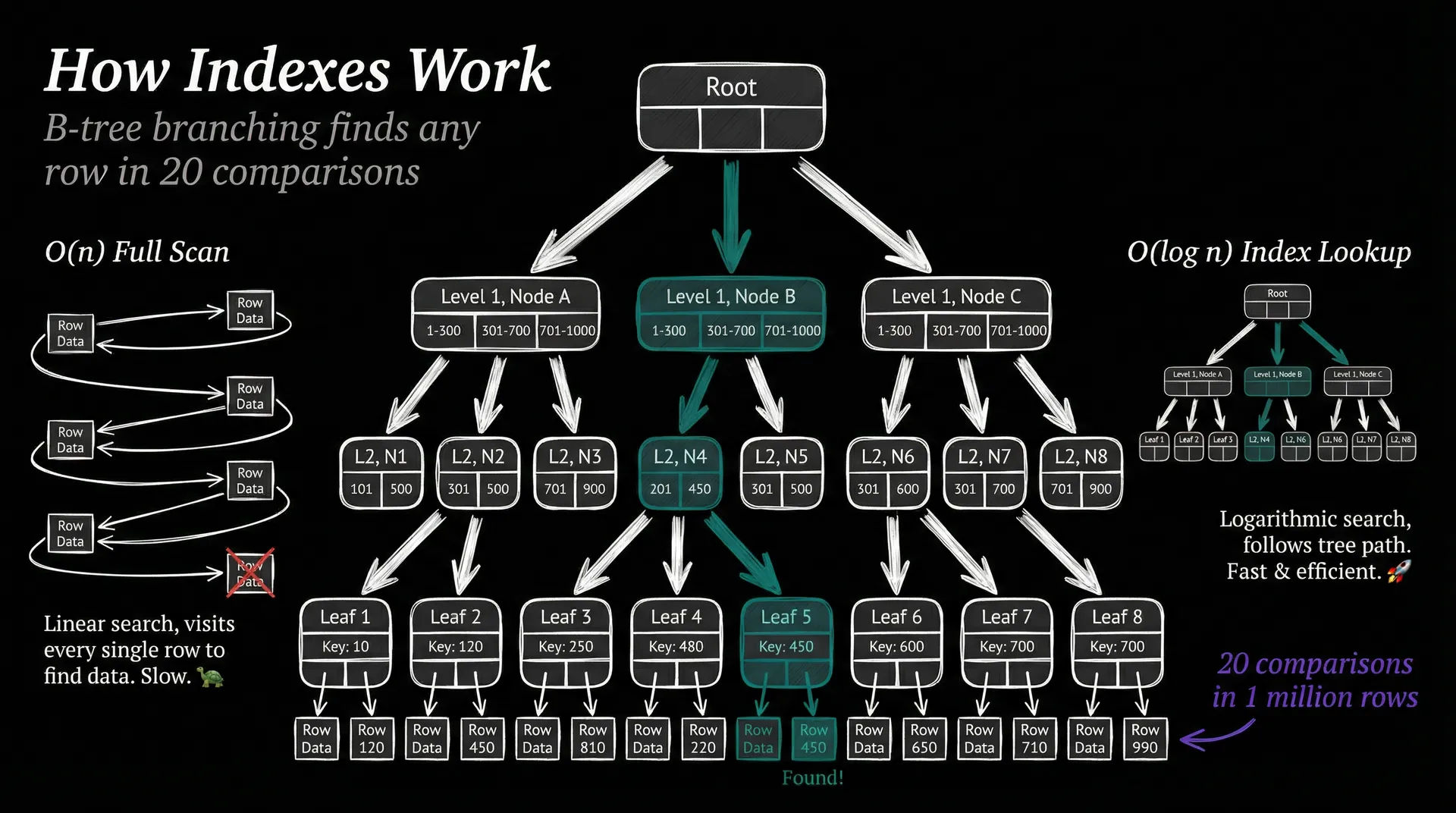
An index works the same way as the index at the back of a textbook: instead of reading every page, you jump straight to the relevant entry. Under the hood, it pre-sorts values into a tree structure called a B-tree. Each node branches into multiple children, so the height stays shallow even as data grows.
Twenty comparisons to find one value in a million rows. That is O(log n), the same runtime as binary search from last article. Pretty remarkable.
The trade-off? Indexes consume disk space and slow writes slightly, because every insert or update must also update the tree. Engineers add indexes deliberately, on the columns they actually query. It is a classic engineering choice: spend a little more on writes to save enormously on reads.
NOT EVERYTHING FITS IN A TABLE
Relational databases are powerful, but they assume your data has a fixed, predictable shape. Sometimes it does not.
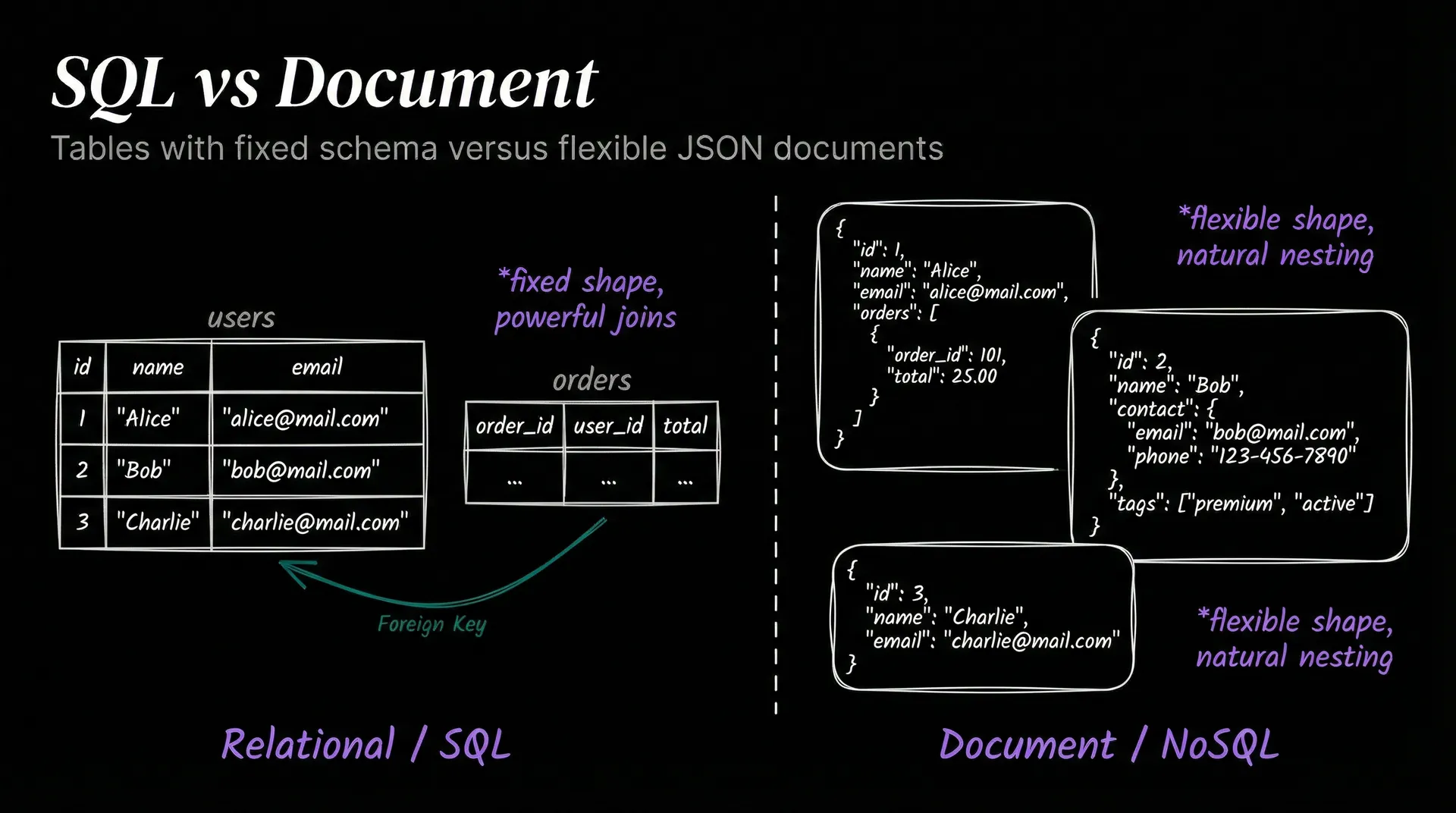
Document databases like MongoDB store data as flexible JSON-like objects. A user profile can have five fields in one document and fifteen in another, no schema required. This works well for content that varies: blog posts, product catalogs, user preferences. The downside is that complex relationships between documents get awkward fast.
Key-value stores like Redis are even simpler. A key maps to a value. That is the whole model.
Redis keeps everything in memory, so reads and writes happen in microseconds. Session tokens, rate-limit counters, and caches are natural fits. Honestly, Redis is one of those tools you reach for constantly once you know it exists.
Graph databases like Neo4j model data as nodes and edges, making relationships first-class citizens. Picture a social network where “Alice follows Bob who follows Carol.” That is a graph problem. Querying three-degree connections in a relational database requires ugly recursive SQL; in a graph database it reads almost like plain English.
VECTOR SEARCH: THE AI-NATIVE DATABASE
Standard databases answer exact questions: give me the row where id = 42. Vector databases answer a fundamentally different one: give me the ten rows most similar to this query. That shift matters enormously for AI.
When a language model processes text, it converts words and sentences into long lists of numbers called vectors. Similar concepts end up near each other in that numeric space.
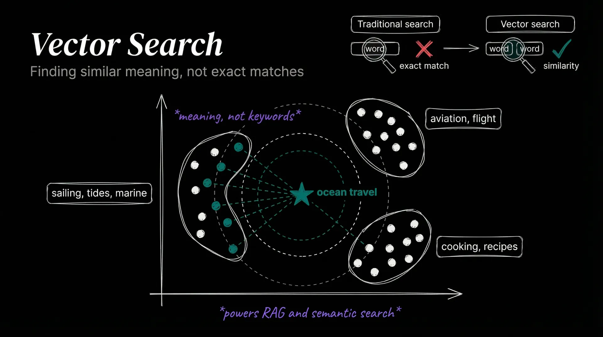
A vector database stores those numbers and answers nearest-neighbor queries: given a new vector, return the stored vectors closest to it.
Imagine a library that shelves books not by title but by meaning. Searching for “ocean travel” surfaces results about sailing, tides, and marine biology even if none of them contain those exact words. That is what vector search does.
This powers retrieval-augmented generation (RAG), the technique that lets AI assistants search a knowledge base before answering. It also drives semantic search, recommendation engines, and duplicate detection. The rise of vector databases like Pinecone and pgvector is a direct consequence of AI going mainstream.
Data storage has come a long way from filing cabinets. Where does all this carefully organized information go next? Article 11 introduces machine learning, the layer where computers start finding patterns in it.
T.
References
-
PostgreSQL: Index Types - Official docs on B-tree and other index types.
-
MongoDB: Document Databases - Overview of the document model and when to use it.
-
Redis: Introduction - Key-value model, data structures, and in-memory architecture.
-
Pinecone: Vector Databases - Vector embeddings, similarity search, and RAG explained.
-
CMU 15-445: Database Internals - Carnegie Mellon’s free database course covering B-trees in depth.