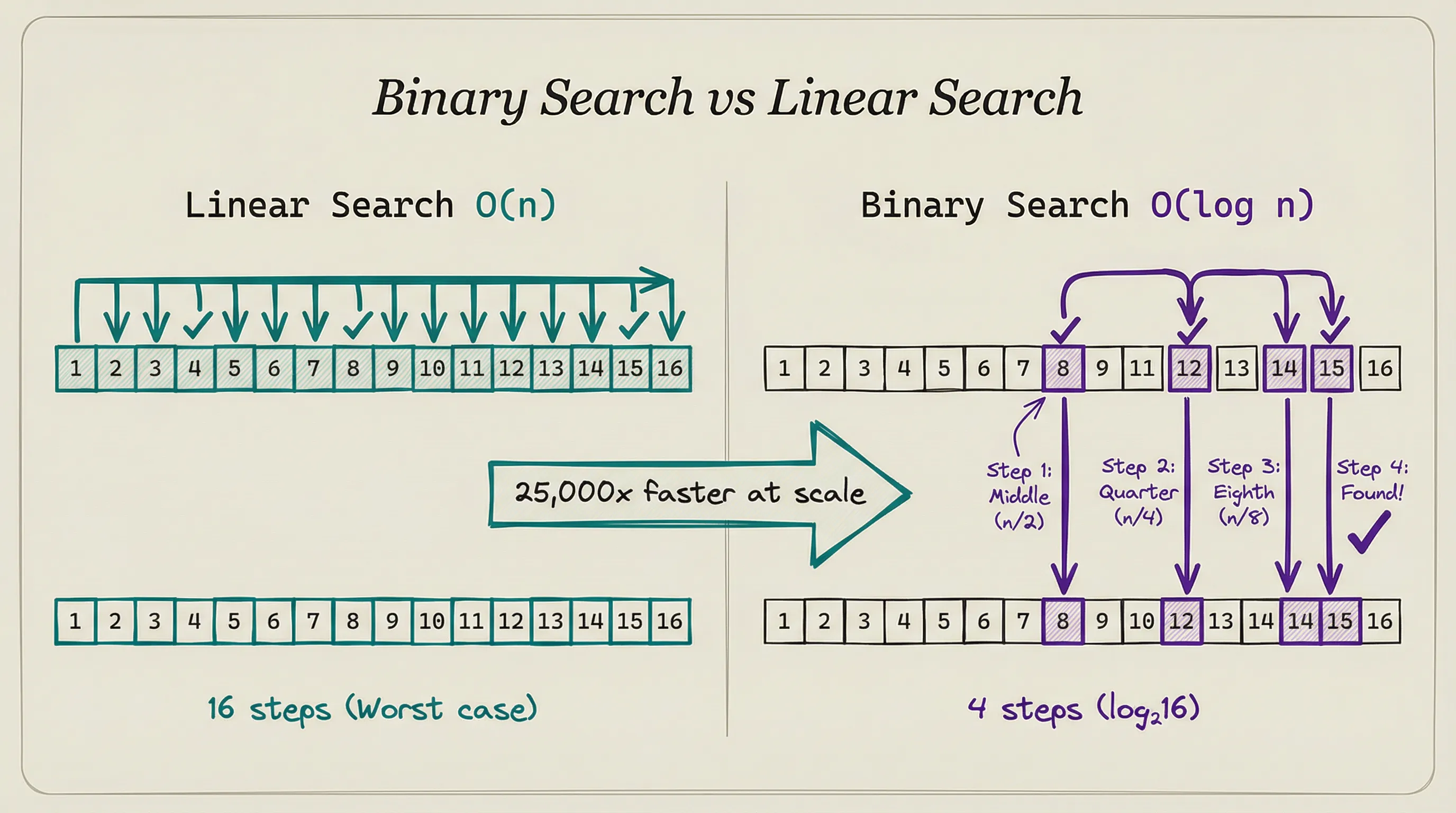
You have a phone book with a million names. You need to find Smith. You could start at page one and check every name until you find it. That might take 500,000 checks on average.
Or you could open the book to the middle, see if Smith comes before or after that page, and cut the remaining pages in half. Repeat. You find Smith in about 20 checks.
Same problem. Same data. Two approaches that differ by a factor of 25,000. That’s the power of choosing the right algorithm.

In Article 8, we covered how code becomes a running program. This article covers something more fundamental: how you decide what the code should do.
An algorithm is a precise set of steps for solving a problem. The choice of algorithm often matters more than the choice of programming language, hardware, or framework.
ALGORITHMS ARE RECIPES (BUT PRECISE)
Think of an algorithm like a cookie recipe. Not a vague mix flour and sugar recipe. A precise recipe.
-
Measure exactly 2.5 cups of all-purpose flour
-
Add exactly 1 cup of butter at room temperature
-
Mix for exactly 3 minutes at medium speed
-
Chill dough for exactly 30 minutes
-
Roll to exactly 0.5 cm thickness
-
Bake at exactly 175°C for exactly 12 minutes
Every step is specific. Every quantity has a definition. The order matters.
Skip step 4 and the cookies spread. Swap steps 3 and 2 and the butter doesn’t incorporate properly.
Algorithms have the same properties:
-
Finite: They end. An algorithm that runs forever is broken.
-
Definite: Each step is unambiguous. Mix well is vague. Mix for 3 minutes at 300 RPM is definite.
-
Input/Output: They take input and produce output. The cookie recipe takes ingredients and produces cookies.
-
Effective: Each step is doable. Solve world hunger is not an algorithm step.
Every program is an algorithm (or a collection of algorithms). The question isn’t whether you need one. It’s whether you chose a good one.
MEASURING SPEED: BIG-O NOTATION
Not all algorithms are equal. Some solve problems quickly. Others take geological time on the same input.
Big-O notation measures how an algorithm’s running time grows as the input size increases. It answers a single question: if I double the input, how much longer does it take?
The phone book example:
Linear search (check every name) is O(n). If the phone book has n names, you might check up to n names. Double the names, double the time.
Binary search (split in half each time) is O(log n). If the phone book has n names, you need at most log₂(n) checks.
A million names takes 20 checks. A billion names takes 30 checks.
Double the names, add just one more check.
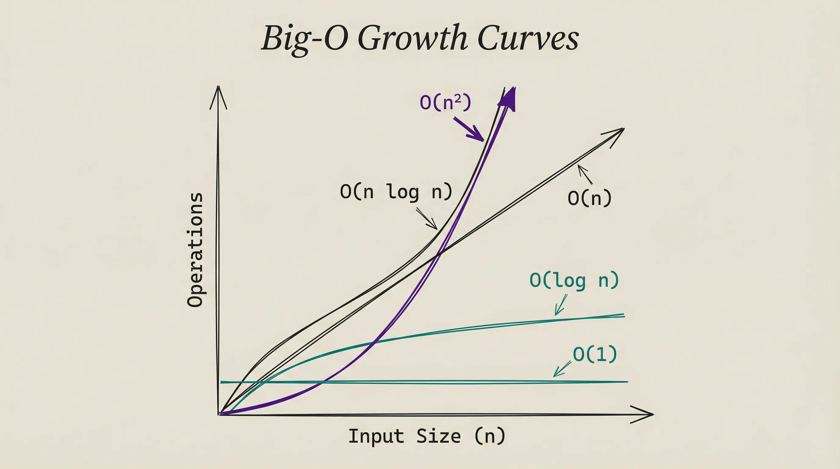
Here’s how different Big-O classes scale:
| Input Size | O(1) | O(log n) | O(n) | O(n log n) | O(n²) |
|---|---|---|---|---|---|
| 10 | 1 | 3 | 10 | 33 | 100 |
| 1,000 | 1 | 10 | 1,000 | 10,000 | 1,000,000 |
| 1,000,000 | 1 | 20 | 1,000,000 | 20,000,000 | 1,000,000,000,000 |
Look at the O(n²) column. For a million items, that’s a trillion operations. Even at a billion operations per second, that takes 16 minutes.
O(n log n) on the same input takes 0.02 seconds.
O(1) means constant time. Looking up an item in a hash table takes the same time whether the table has 10 entries or 10 million. The input size doesn’t matter.
O(n²) means quadratic time. Double the input, quadruple the time. Comparing every item against every other item is O(n²). This is why naive approaches break at scale.
SORTING: THE CLASSIC EXAMPLE
Sorting is the most studied problem in computer science. Put a list of items in order. Simple goal, dozens of approaches, wildly different performance.
BUBBLE SORT: THE NAIVE APPROACH
Compare adjacent items. If they’re in the wrong order, swap them. Repeat until nothing swaps.
For a list of 10 items, this works fine. For a million items, bubble sort is O(n²): roughly a trillion comparisons. It’s the algorithm equivalent of checking every combination.
Nobody uses bubble sort in production. But it illustrates why algorithm choice matters.
QUICKSORT: DIVIDE AND CONQUER
Pick a pivot element. Move everything smaller to the left, everything larger to the right. Now you have two smaller lists. Repeat on each sub-list.
Quicksort is O(n log n) on average. For a million items: about 20 million operations instead of a trillion. That’s 50,000 times faster than bubble sort on the same data.
The divide and conquer strategy is powerful: break a big problem into smaller problems, solve those, combine results. Many efficient algorithms follow this pattern.
WHY SORTING MATTERS FOR AI
AI systems sort and rank constantly. Search results need ranking. Recommendation systems sort candidates by predicted preference. Attention mechanisms in transformers compute similarity scores and pick the highest ones.
The difference between O(n²) and O(n log n) at AI scale (millions to billions of items) is the difference between seconds and days.
SEARCH: FINDING WHAT YOU NEED
LINEAR SEARCH
Check every item until you find the target. O(n). Works on unsorted data. Simple but slow for large datasets.
BINARY SEARCH
Requires sorted data. Check the middle element.
If the target is smaller, search the left half. If larger, search the right half. O(log n).
This is the phone book example. Binary search is the reason sorted data is so valuable. Sorting costs O(n log n) up front, but after that every search takes O(log n) instead of O(n).
HASH TABLES
Store each item at a location determined by its key. A hash function converts the key into an array index.
Looking up Smith computes hash(Smith) = 47392, then checks position 47392 directly. O(1) average case.
Hash tables power most software: Python dictionaries, JavaScript objects, database indexes, caching systems. When you hear constant-time lookup, it\u2019s usually a hash table.
The trade-off: hash tables use more memory than arrays, and they don’t maintain order. If you need sorted data, a hash table won’t help. But for pure lookup speed, nothing beats them.
TREES
Binary search trees maintain sorted order while allowing fast insertion and lookup. Each node has at most two children: left (smaller values) and right (larger values). Searching takes O(log n) on a balanced tree.
Databases use a variant called B-trees (Article 10 covers this in depth). B-trees optimize for disk access, storing multiple keys per node to minimize the number of disk reads needed to find a value.
GRAPH ALGORITHMS: NAVIGATING NETWORKS
Not all problems involve simple lists. Many real-world systems form graphs: networks of connected nodes.
Social networks are graphs. Each person is a node, each friendship is an edge.
The internet is a graph (Article 7). Routers are nodes, cables are edges. Road maps are graphs. Intersections are nodes, roads are edges.
SHORTEST PATH
When Google Maps finds the fastest route, it runs a graph algorithm. Dijkstra’s algorithm finds the shortest path between two nodes by exploring outward from the starting point, always choosing the nearest unvisited node next.
GPS navigation, network routing (BGP from Article 7), and logistics optimization all use shortest-path algorithms. Every time Google Maps recalculates your route in traffic, it runs a version of Dijkstra’s algorithm on a graph with millions of road segments.
PAGERANK
Google’s original search algorithm treated the web as a graph. Each page is a node, each hyperlink is an edge. PageRank computed each page’s importance based on how many important pages linked to it.
This recursive definition (importance depends on the importance of connected pages) made web search dramatically better than keyword matching alone. The algorithm that built Google was a graph algorithm.
ALGORITHMS THAT POWER AI
Several algorithms are particularly important for understanding AI.
GRADIENT DESCENT
Training a neural network means finding the weights (parameters) that minimize errors. The search space has billions of dimensions (one per parameter). You can’t check every possibility.
Gradient descent is like finding the lowest point in a mountain range while blindfolded. You feel the slope under your feet and take a step downhill. Repeat. You can’t see the terrain around you, but you can always find down from where you stand.
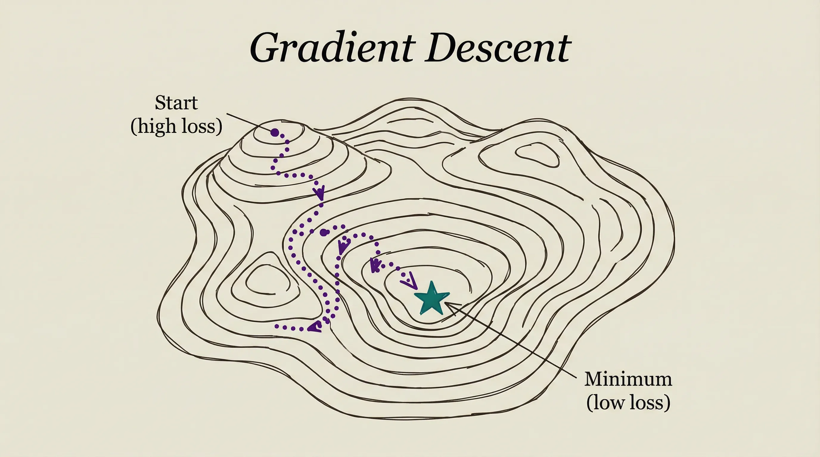
Mathematically, the gradient is the direction of steepest increase. Move in the opposite direction (steepest decrease) and you reduce the error. Each step adjusts millions or billions of parameters by a tiny amount.
The learning rate determines step size. Too large and you overshoot valleys. Too small and training takes forever. Finding the right learning rate is one of the key challenges in training AI models.
BACKPROPAGATION
Backpropagation calculates the gradient efficiently. A neural network has many layers. Backpropagation starts at the output (the error), then works backward through each layer, computing how much each weight contributed to the error.
This backward pass enables gradient descent to work on deep networks. Without backpropagation, training networks with hundreds of layers would be computationally impractical.
ATTENTION MECHANISM
The attention algorithm (from the 2017 Attention Is All You Need paper) powers every modern large language model. It lets the model weigh the importance of different input tokens relative to each other.
For every token in the input, attention computes a score against every other token. The computation is O(n²) where n is the sequence length. This is why LLMs have context length limits and why longer prompts cost more to process.
Researchers actively work on reducing attention’s quadratic cost. Techniques like sparse attention, linear attention, and sliding window attention bring the cost closer to O(n), enabling longer context windows.
WHY THIS MATTERS
Algorithm choice determines what’s computationally feasible.
Why some AI models are faster: Model architecture choices (Article 13 will cover this in depth) are algorithm choices. A model with efficient attention is faster than one with standard attention, even on the same hardware.
Why preprocessing data matters: Sorting, indexing, and structuring data before processing it enables faster algorithms. A database with proper indexes (Article 10 covers this) uses binary search instead of linear search.
Why scale creates new problems: An algorithm that works fine on 1,000 items might be unusable on 1 billion items. O(n²) on a billion items requires 10¹⁸ operations. That’s about 30 years of computation on a single core.
Why optimization is a field: Gradient descent isn’t the only optimization algorithm. Adam, SGD with momentum, AdaFactor, and others each trade off speed, memory, and convergence. Choosing the right optimizer affects training time and model quality.
The right algorithm turns impossible into trivial. The wrong one turns trivial into impossible.
WHAT’S NEXT
Algorithms process data. But where does that data live? How do systems store, organize, and retrieve billions of records efficiently?
In Article 10, we’ll look at databases: the systems that store everything from your social media posts to the training data that teaches AI models. Indexes, queries, transactions, and the new category of vector databases purpose-built for AI.
T.
REFERENCES
-
Introduction to Algorithms (CLRS) - The standard reference textbook for algorithms and data structures
-
Big-O Cheat Sheet - Visual reference for algorithm time complexities
-
Attention Is All You Need (Vaswani et al, 2017) - The transformer paper that introduced the attention mechanism
-
Visualizing Algorithms - Mike Bostock - Interactive visualizations of sorting and search algorithms
-
Gradient Descent Optimization Algorithms - Overview of optimization algorithms used in deep learning