The previous article ended with a matrix: one row per token, each row a dense vector of floating-point numbers. The embedding matrix looked up each token ID and returned that vector. The text was gone. What remained was geometry.
But something was still missing.
Those vectors carry meaning, but they carry no position. The embedding for bank is the same whether it appears first in the sentence or last. The vector for not is identical whether it negates the word before it or the word after it.
Feed that matrix into the attention mechanism from article three, and you get a model that cannot tell the dog bit the man from the man bit the dog. Both sentences contain the same tokens. Attention treats them identically.
This is not a bug. It is a mathematical property of attention. Attention is, by design, permutation invariant: shuffle the input tokens into any order and the computation produces the same result.
That property makes attention efficient and parallelizable. The transformer has to add position back in deliberately.
Positional encoding is how the transformer does it. And once the transformer handles position, there is still one more problem to solve at the other end: how does the model decide what word to say? That question belongs to sampling, and this article covers both.
THE PROBLEM WITH ORDER
Before attention existed, recurrent networks processed tokens one at a time, left to right. The architecture built position into itself. The network arrived at token one, then token two, then token three. The sequence of arrival was the position signal.
Attention throws that out. It processes all tokens simultaneously, comparing every token against every other token in parallel. That is its great advantage over recurrent models. But parallel processing carries no inherent sense of order.
Think of it like a library where every book arrives at once, face-down on a table. You can flip them all over and compare them at the same time. But to know which book came out first, someone has to have stamped a date inside the cover. Attention needs the same thing: a mark on each token that says where it came from.
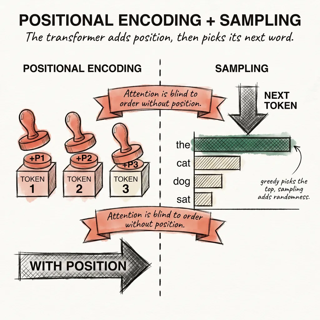
The fix is simple. Add a positional signal directly to each token embedding, before passing anything to attention. Not a separate input. Just a vector added to the embedding vector already sitting in each row of the matrix.
The embedding says what the token means. The positional vector says where it sits. Together they give attention what it needs.
SINE AND COSINE
The original transformer paper introduced a specific formula for generating positional vectors. It uses sine and cosine functions at different frequencies, one per dimension of the embedding vector.
For a token at position p in the sequence, and for each dimension i of the embedding:
- Even dimensions: sin(p / 10000^(2i / d))
- Odd dimensions: cos(p / 10000^(2i / d))
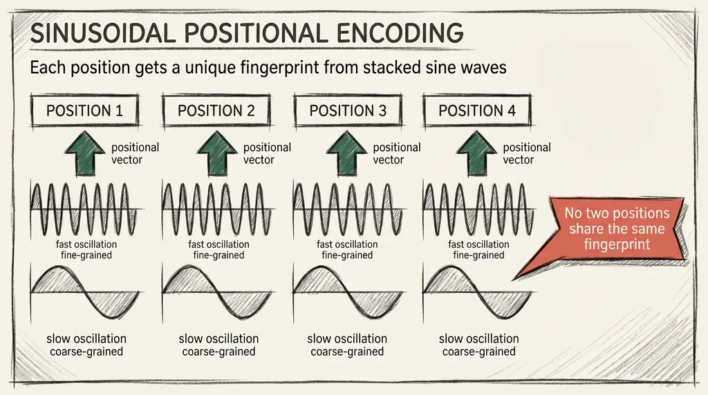
Where d is the embedding dimension. The large base of 10000 creates a very wide range of frequencies. Low-numbered dimensions oscillate quickly and encode fine-grained position. High-numbered dimensions oscillate slowly and encode coarse-grained position.
Together they create a unique fingerprint for each position in the sequence, like the hands of a clock at different scales: seconds, minutes, hours. No two positions share the same fingerprint.
The transformer adds this fingerprint to the token embedding. Attention can then distinguish bank at position 2 from bank at position 14, because those two instances now carry different vectors.
I find the sinusoidal choice interesting because it is not the obvious one. The researchers could have just assigned each position an integer. They chose trigonometric functions partly because the encoding for position p + k can be expressed as a linear transformation of the encoding for position p.
The model can learn to attend to three positions ahead without anyone teaching it offsets explicitly. The geometry captures relative position as a side effect.
LEARNED VS. FIXED
Sinusoidal encoding is static. You compute it once from the formula and it never changes during training. This is convenient. It is also limiting, because the formula knows nothing about what the model is learning.
The alternative treats positional encodings as parameters. Each position gets its own vector, initialized randomly, adjusted by gradient descent over the course of training. Over millions of examples, the model shapes those vectors to encode whatever positional information turns out to matter.
GPT-2, GPT-3, and most large language models use learned positional embeddings rather than fixed ones. For positions within the training range, the practical difference is small.
At the edges the gap shows: familiar positions have adapted through exposure, while positions outside the training range have not.
Both approaches share the same structure: a vector added to each token embedding before attention runs. The question is only whether that vector comes from a formula or from the data.
WHY RELATIVE POSITION MATTERS
Fixed and learned embeddings share a deeper limitation. Both tie each position’s vector to an absolute index. Position 1 gets one vector, position 500 gets another.
The model must learn that subject at position 1, verb at position 3 and subject at position 500, verb at position 502 express the same grammatical relationship. That is harder than it sounds.
This is why most modern large language models use Rotary Position Embedding, or RoPE. Instead of adding a positional vector to each embedding, RoPE rotates the query and key vectors by an amount proportional to their position. The rotation makes the dot product between any query and any key depend only on their relative distance.
A query at position 5 and a key at position 8 interact the same way as a query at position 105 and a key at position 108. The three-position gap is what matters, not where in the sequence that gap falls.
LLaMA, Mistral, and most 2024–2025 models use RoPE. The original sinusoidal approach is now mostly of historical interest, though understanding it is the fastest path to understanding why its successors look different.
THE OTHER END: SAMPLING
Once the transformer adds positional encoding and runs all its attention layers, it has built a rich representation of your prompt. Now it has to produce an answer, one token at a time.
The final attention layer produces an internal state vector. A linear layer maps that vector down to the size of the vocabulary: one score per possible next token. These raw scores are logits.
A softmax function converts the logits into a probability distribution: every score falls between 0 and 1 and all scores sum to 1. The model picks the next token by sampling from that distribution.
The simplest strategy is greedy decoding: always pick the highest-probability token. Greedy decoding is deterministic and fast, but it produces repetitive, sometimes boring output. It gets stuck in loops.
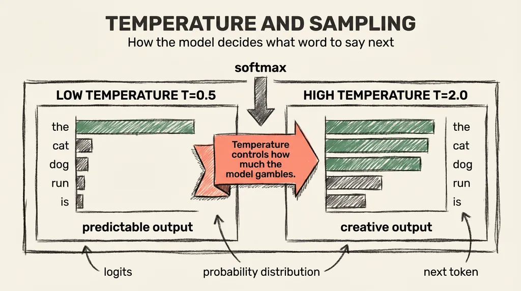
Temperature is the first adjustment. Before applying softmax, divide all the logits by a number T. At T = 1, the distribution stays unchanged. At T < 1, high-probability tokens grow even more dominant and the distribution sharpens.
At T > 1, the distribution flattens and unlikely tokens become more competitive. Think of it like a price auction. Low temperature makes the frontrunner almost certain to win. High temperature brings in more competitors and makes the outcome harder to predict.
Honestly, I think temperature is the most underrated control in AI tooling. Most people treat it as an exotic dial. It is actually just telling the model how much to gamble.
Top-p sampling, also called nucleus sampling, adds a constraint on top of temperature. After sorting tokens by probability, keep only the smallest set of tokens whose cumulative probability exceeds threshold p. Sample from that set only.
At p = 0.9, the model ignores any token outside the top 90% of probability mass. This cuts the long tail of implausible continuations without artificially capping the number of candidates.
Top-k sampling is simpler: keep the k highest-probability tokens, sample from those. At k = 50, the model chooses among its 50 best guesses.
In practice, most systems combine temperature with top-p. Temperature reshapes the distribution first, then top-p clips the tail. The result is output that is creative without becoming incoherent.
THE COMPLETE PICTURE
Here is the full pipeline, from your prompt to the model’s reply.
Your text enters the tokenizer, which breaks it into tokens and maps each to an integer ID. The embedding matrix looks up each ID and returns a dense vector. Positional encoding adds a position fingerprint to each vector.
The enriched matrix enters the stack of attention layers. Each layer refines the representation. The final layer’s output passes through a projection to produce logits.
Temperature and top-p reshape the distribution. The model samples one token and feeds it back in as input. The whole thing repeats until the model produces a stop signal.
Every article in this act covered one step in that pipeline. Tokens and embeddings were the input stage. Attention was the processing core.
Positional encoding was the fix for order. Sampling is the output mechanism.
The next act covers what shapes the model around that pipeline: context windows, parameter counts, scaling laws, Mixture of Experts, and the design decisions that determine what a model can and cannot do. The pipeline stays the same. The constraints around it change everything.
T.
References
-
Attention Is All You Need (Vaswani et al., 2017) - The original transformer paper. Section 3.5 describes sinusoidal positional encoding and the mathematical properties that motivated the choice of sine and cosine over learned embeddings.
-
RoFormer: Enhanced Transformer with Rotary Position Embedding (Su et al., 2021) - The paper introducing RoPE, which encodes position as a rotation of query and key vectors. Now the standard approach in LLaMA, Mistral, and most modern large language models.
-
Language Models are Few-Shot Learners (Brown et al., 2020) - The GPT-3 paper. Section 2.1 describes the architecture, including the choice of learned positional embeddings over the original sinusoidal approach.
-
The Curious Case of Neural Text Degeneration (Holtzman et al., 2019) - The paper that introduced nucleus sampling. Demonstrates why greedy decoding and top-k sampling produce degenerate text, and proposes the cumulative probability threshold that most production systems now use.
-
Train Short, Test Long (Press et al., 2021) - Introduces ALiBi, which adds a learned bias to attention scores rather than modifying embeddings. Shows that generalizing to longer sequences than seen during training is an active research problem with multiple viable approaches.