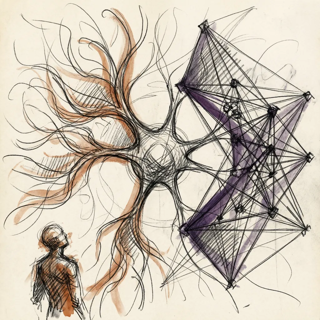
Your brain has 86 billion neurons. Each one connects to thousands of others through synapses. A neuron receives signals from its neighbors, and if those signals are strong enough, it fires its own signal to the next set of neighbors.
That’s biological intelligence. Artificial neural networks take the same core idea, strip it down to pure math, and run it on GPUs.
In Article 11, we covered machine learning: computers finding patterns in data. Neural networks are a specific type of machine learning model. They’re the type that powers large language models, image generators, self-driving cars, and virtually every AI system making headlines in 2026.
The Voting Committee Analogy
Think of a neural network as a voting committee.
You’re trying to decide whether a photo contains a cat. Each committee member (neuron) looks at a small piece of evidence and casts a weighted vote. One member checks for pointy ears. Another checks for whiskers.
Another checks for fur texture. No single vote determines the answer. The committee combines all votes, weighted by each member’s reliability, to reach a decision.
Members who have been right in the past get more influence. Members who have been wrong get less.
Training the network means adjusting the voting weights. After thousands of photos, the committee learns which features matter for cat versus not cat. Some members become experts at detecting ears. Others become useless and get near-zero weight.
Stack multiple committees in layers, where one committee’s output becomes the next committee’s input, and you get a deep neural network.
The Artificial Neuron
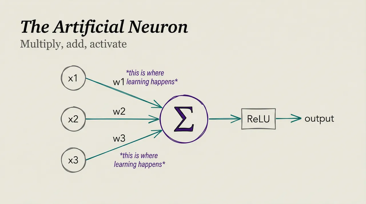
A biological neuron receives inputs, processes them, and produces an output. An artificial neuron does the same thing with simple math. Think of it like a tiny calculator with a dial: it takes in numbers, does one operation, and passes the result along.
Each artificial neuron does five things. It receives inputs (numbers) from connected neurons. It multiplies each input by a weight (how important that connection is). It adds up all the weighted inputs, adds a bias (a constant that shifts the result), and passes the sum through an activation function that determines if the neuron fires.
In math: output = activation(w₁x₁ + w₂x₂ + w₃x₃ + … + bias)
That’s it. Multiply, add, activate. Every artificial neuron does only this.
The power comes from connecting millions of them together. The same way individual ants follow simple rules, yet the colony solves complex problems.
Activation Functions: Why Nonlinearity Matters
The activation function is what makes neural networks powerful. Without it, a neural network would just be a series of multiplications and additions, which simplifies to a single linear transformation. A straight line.
A straight line can’t model curved relationships. “Houses near the city center cost more” isn’t linear. Houses very close to the center might cost less (noise, congestion). The relationship curves.
Activation functions act like bouncers at a nightclub. They decide what gets through and what gets blocked, shaping the signal before it moves to the next layer.
ReLU (Rectified Linear Unit) is the most common activation function. If the input is positive, output it unchanged. If negative, output zero.
Sigmoid squashes any input to a value between 0 and 1. Useful for outputs that represent probabilities, like estimating a 0.87 chance an email is spam.
Softmax takes a vector of numbers and converts them to probabilities that sum to 1. The output layer uses it for classification, assigning each category a probability like 85% cat, 10% dog, 5% bird.
The activation function introduces nonlinearity, which lets the network model complex, curved relationships. Stack enough nonlinear layers and a neural network can approximate any mathematical function. This is the universal approximation theorem, and it’s why neural networks are so flexible.
Layers: Building Depth
A neural network arranges neurons into layers:
Input layer. Receives the raw data. For an image, each pixel value becomes one input neuron. A 224x224 color image has 150,528 input neurons (224 x 224 x 3 color channels).
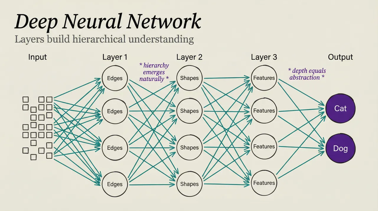
Hidden layers. Process and transform the data. Each hidden layer learns to detect progressively more abstract features. The first hidden layer might detect edges, the second detects shapes, the third detects parts (ears, whiskers), and the fourth detects objects (cat, dog).
Output layer. Produces the final answer. For classification, one neuron per category. For regression, a single neuron with the predicted value.
A network with many hidden layers is a deep neural network. This is where deep learning gets its name. Depth lets the network build hierarchical representations: simple features combine into complex features that combine into abstract concepts.
How many layers? Frontier language models likely have 120+ transformer layers. Each layer refines the representation, making it more useful for the final task.
Training: Backpropagation
We covered gradient descent in Article 9: take a step in the direction that reduces error. But in a network with millions of parameters across dozens of layers, how do you know which parameters to adjust and by how much?
Backpropagation solves this. It calculates the gradient (direction of steepest error increase) for every parameter in the network by working backward from the output layer. Think of it like tracing a plumbing leak backward through the pipes. You start at the puddle (the error) and follow the connections back to find which joints (weights) need tightening.
The process works in four steps. First, the forward pass feeds an input through the network, layer by layer, to produce a prediction. Second, the loss calculation compares the prediction to the correct answer. The difference measures the error.
Third, the backward pass starts at the output and calculates how much each weight contributed to the error, using the chain rule from calculus to propagate this signal backward through every layer. Finally, the weight update adjusts each weight proportional to its contribution to the error.
This happens for every training example. After millions of examples, the weights converge to values that produce good predictions.
The math is elegant: the chain rule lets you decompose a complex function into simple pieces, calculate the gradient for each piece, and multiply them together. This makes training deep networks computationally tractable. Without backpropagation, training a 100-layer network would require brute-force search through billions of dimensions.
Why More Layers Help
A single-layer network can only learn linear relationships. Two layers can learn simple curves. But real-world patterns are deeply hierarchical.
Consider recognizing a face. Layer 1 detects edges (horizontal, vertical, diagonal lines). Layer 2 combines edges into textures and simple shapes. Layer 3 combines shapes into facial features (eyes, nose, mouth).
Layer 4 combines features into faces. Layer 5 identifies specific individuals.
Each layer builds on the previous one. Layer 4 doesn’t need to learn what an edge is. It receives pre-processed feature information from layers 1–3 and focuses on combining them.
This hierarchy emerges naturally during training. Nobody programs “detect edges in layer 1.” The network discovers that edge detection is useful for the task and organizes itself accordingly.
Network Architectures
Different problems need different network shapes. Just as you wouldn’t use a hammer to turn a screw, each architecture fits a particular kind of data.
Convolutional Neural Networks (CNNs)
CNNs process images by sliding small filters across the image, like a magnifying glass scanning a photograph one patch at a time. Each filter detects a specific pattern (edge, corner, texture). The filter shares weights across the entire image, so a pattern detector trained in one location works everywhere.
CNNs power image recognition, medical imaging, self-driving car vision, and facial recognition. They work because images have spatial structure: nearby pixels relate to each other.
Recurrent Neural Networks (RNNs)
RNNs process sequences one element at a time, maintaining a hidden state that carries information from previous elements. When processing “The cat sat on the ___”, the hidden state accumulates context from each preceding word.
RNNs dominated language tasks before 2017. They struggled with long sequences because information degraded as it passed through many time steps. LSTMs (Long Short-Term Memory) networks added gates to control information flow, partially solving this problem.
But even LSTMs couldn’t handle very long sequences well. Enter transformers.
Transformers: The Architecture That Changed Everything
In 2017, the paper “Attention Is All You Need” introduced the transformer architecture. Instead of processing sequences one element at a time (like RNNs), transformers process all elements simultaneously and use attention to determine which elements are relevant to each other.
Attention answers: “When processing word X, how much should I focus on each other word in the input?”
Consider the sentence: The cat sat on the mat because it felt tired. When the model processes the word it, the attention mechanism links it most strongly to cat. Matrix multiplication (Article 4) drives this connection, not explicit rules.
Transformers dominate AI in 2026. Language models, image generators, speech recognition systems, and protein structure prediction tools all use transformer architectures. The architecture scales, parallelizes efficiently on GPUs, and captures long-range dependencies that earlier designs couldn’t.
The transformer succeeded because it processes all tokens in parallel (GPU-friendly, unlike sequential RNNs). Attention captures long-range dependencies, unlike RNNs that forget distant context. And it scales predictably: more parameters and data consistently improve performance.
Article 13 will break down transformers and LLMs in full detail.
How Big Are Modern Networks?
| Model | Parameters | Architecture | Year |
|---|---|---|---|
| AlexNet | 60 million | CNN | 2012 |
| BERT | 340 million | Transformer | 2018 |
| GPT-3 | 175 billion | Transformer | 2020 |
| GPT-4 | ~1.8 trillion (estimated) | Transformer (MoE) | 2023 |
| Llama 3 405B | 405 billion | Transformer | 2024 |
| DeepSeek-V3 | 671 billion (37B active) | Transformer (MoE) | 2025 |
| Llama 4 Maverick | 400 billion (17B active) | Transformer (MoE) | 2025 |
A parameter is a single weight or bias in the network. GPT-4’s estimated 1.8 trillion parameters means 1.8 trillion numbers training adjusted to minimize prediction error.
The 2025 models reveal a new pattern: Mixture of Experts (MoE) architecture. DeepSeek-V3 has 671 billion total parameters, but only 37 billion activate for any given input. The network routes each token to specialist sub-networks.
More total knowledge, less active compute per query. It’s the difference between hiring a thousand specialists and consulting three of them per problem.
Training stores each parameter as a number (typically 16 bits). A model with 671 billion parameters takes over 1 terabyte of storage. Running it requires GPU clusters with terabytes of combined memory, which is why frontier AI runs in data centers, not on your laptop.
Why This Matters
Neural networks are the core technology behind modern AI. Understanding them explains:
Why AI is expensive. Training adjusts billions of parameters across trillions of data points. Each adjustment requires GPU computation. Scale the parameters and data, and costs scale with them.
Why AI has patterns. Neural networks learn statistical patterns from training data. They don’t understand in the human sense. They find correlations.
This explains both their impressive capabilities and their strange failures (confidently stating wrong facts, for example).
Why architecture matters. CNNs for images, transformers for language. The network shape determines what patterns it can learn efficiently.
Why scaling works. Larger networks with more data consistently perform better. This empirical observation (called scaling laws) drives the industry’s appetite for more GPUs, more data, and bigger models.
What’s Next
Neural networks are the engine. But the specific type of neural network that powers AI chatbots is the Large Language Model (LLM).
In Article 13, we’ll zoom into exactly how LLMs work. How text becomes numbers. How attention lets models understand context. And how predicting the next word, trillions of times, produces something that looks like intelligence.
T.
References
-
3Blue1Brown - Neural Networks - Visual introduction to how neural networks learn
-
Attention Is All You Need (Vaswani et al, 2017) - The paper that introduced the transformer architecture
-
Stanford CS231n - CNNs for Visual Recognition - Stanford course covering convolutional neural networks
-
Universal Approximation Theorem - Proof that neural networks can approximate any continuous function
-
Scaling Laws for Neural Language Models (Kaplan et al, 2020) - Research on model size, data, compute, and performance
-
Machine Learning: How Computers Learn (Article 11) - Previous article on machine learning fundamentals